-
How much heat ?
We present a quick simulation study on the Raspberry
 B+. First, we estimate the power dissipation using our power budget calculator from a previous blog (>>click here<<). We impose the following conditions: ambient temperature of 25 ºC and housing temperature of 40 ºC, this is the maximum allowable touch temperature at the external surfaces of the housing. The dimensions used for the housing are: length 89.5 mm, width 61 mm, and height 24 mm.
The calculator returns a value of 3.3 W. However, the estimated power consumption during heavy workload is 1.76 W.
As the predicted power dissipation is 3.3 W and we only expect to dissipate 1.76 W there should be no thermal issues. We will see …
Then, we create a detailed model of the Raspberry
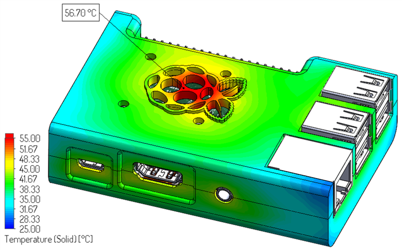
B+ and applied 3.3 W to the unit to corroborate the results from our calculator. The results are shown in the picture below.
It is clear that there is a significant discrepancy between the first order approximation (our calculator) and the simulation model. Why? Well, the power budget calculator assumes that all external surfaces dissipate heat at a uniform temperature. Obviously, that is not the case in a real system. Exemplified by the hot spot on the top-housing at the location of the raspberry structure (logo); otherwise all surfaces should look at the same color.
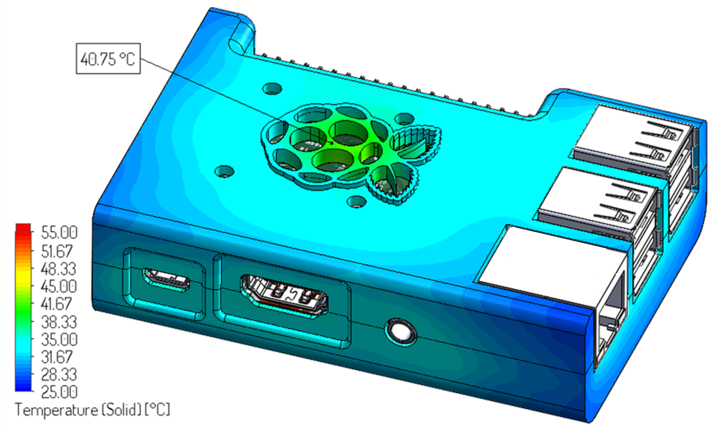
We know that the unit cannot dissipate 3.3 W but then we check that at least the unit is meeting the housing limit of 40 ºC during heavy workload at 1.76 W. The results are shown in the figure below.
The new simulation shows that the unit meets the housing temperature limit at the specified power consumption (1.76 W @ 40 ºC). Because the results show an exact match to the housing temperature of 40 ºC, the power budget calculation can be adjusted by a cooling-efficiency (
 ), and use it in future calculations. The simplest efficiency can be calculated as:
![\[ \eta_{cool}=\frac{P_M}{P_E}, \]](http://www.fluxthermaldesign.com/wp-content/ql-cache/quicklatex.com-bd8291e9eb414e33fdd633baf685e483_l3.png "Rendered by QuickLaTeX.com")
where
 is the measured/real/simulated power and
  is the calculated power using the power budget calculator.
Using the previous equation, we got a cooling efficiency of 50%, indicating how much the housing deviates from the assumption of uniform temperature distribution in all external surfaces.
Let assume for a moment that the engineers of this project realized that the housing limit of 40 ºC is too restrictive. The surface at the location of the hot spot is plastic and with more than a 60% open area ration (reducing contact area). These two observations allow the engineers to increase the housing temperature limit to 45 ºC.
Because the value of
is now known. We go back to the calculator and predict how much power the system can support to meet the new housing limit of 45 ºC.The resulting value is 4.6 W before adjusting it by
and 2.3 W after the adjustment.Finally, we checked at 2.3 W with the detailed simulation model. The results are shown in the figure below.
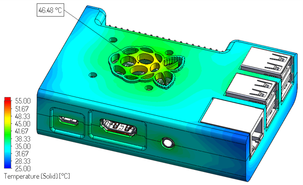
The results from the detailed model showed a very close value of 46.5 ºC to 45 ºC indicating an accurate power budget dissipation from our calculator.
This corroborates that the
value can be used in future calculations if the conditions change.Results from the power budget calculator and even from detailed models are only approximations that can be used to help thermal engineers in the design phase. However, these approximations are based on multiple assumptions that are difficult to replicate in real life. Thus, it is always necessary to check with real measurements that the proposed solutions are working as predicted.
 (1 votes, average: 5.00 out of 5)
 Loading...